
The Cyclistic Bike Share Case Study is from the Coursera Google Analytics Capstone course. The goal of this project was to determine factors that differentiate annual members and casual bike riders. These factors are then used to develop recommendations for a marketing campaign that aims to increase the membership conversion rate.
The tools I used for this project were R and Tableau. Check out the R Script to follow along or head to my Tableau viz story to see the end result!
Scenario
The first quarter of 2020 just came to a close. The marketing team at Cyclistic, a Chicago bike share company, wants to develop a targeted marketing campaign that converts casual customers into members. You have access to historical bikeshare data of the past four quarters (2019 Q2/Q3/Q4 and 2020 Q1).
Stakeholder Goal
Cyclistic aims to increase its number of annual memberships by targeting casual members through a marketing campaign.
Business Task
Using historical data, determine key factors which differentiate casual riders from annual members.
Data Descriptions
The descriptions below are based on Google’s ROCCC analysis. Each description was given a rating of zero to five, five meaning meets expectations.
Reliable: Rating 2/5
The data is located in an aws cloud warehouse in .zip files that are organized by financial quarter. There is currently no encrypted password or user permissions set for these files. An encrypted password or user permissions should be added to the data files to protect the integrity and improve the security of the stakeholder’s data.
Relevant: Rating 4/5
The data is relevant to the business problem. However, gender and birth year columns in the data are either missing or contain nulls. It is recommended that the gender of members is added for a robust analysis on the demographics of Cyclistic Bikes’ customers.
Original: Rating 5/5
The data is proprietary and collected from the original source.
Comprehensive Rating 2/5
The data is organized by trip id and not customer id. This makes it difficult to determine the frequency of bike use per customer. If the same customer makes multiple trips, this can introduce bias into the analysis.
Current: Rating 5/5
The data is current to the case study setting (end of Q1 in 2020).
Cited: Rating 5/5
The data is from a trustworthy source.
Data Preparation
- Set user permissions and/or encrypted file passwords
- Add gender and birth year to all datasets (if attainable)
- Collect or obtain customer ids to determine frequency of users’ trips (if attainable)
Data Processing
For the purpose of this case study, trip ids were counted as individual customers. Here are the steps I used to transform and clean my data in preparation for analysis:
- Standardize column names
- Add a column to 2020 Q1 data for the calculated ‘tripduration’
- Select relevant columns
- Add column to designate quarter-year (ex. Q2_2019)
- Combine dataframes
- Separate DateTime column into Date and Time columns
- Check and change data structures to coorect data type
- Add month, date, year, day of week, and hour columns
- Drop extra date columns
- Remove duplicates and NAs
- Standardize usertypes to match stakeholder definitions
- Remove bikes ‘from HQ’ and negative trip duration values
Not interested in the R-documentation? Skip to analysis summary or the recommendations!
R-Documentation
Data Processing
Make sure to set appropriate working directory. Then load the required packages and data from .csv files.
setwd("path-goes-here")

#Load packages
library(tidyverse)
library(plyr)

#Load data
Divvy_Trips_2019_Q2 <- read_csv("Divvy_Trips_2019_Q2.csv")
Divvy_Trips_2019_Q3 <- read_csv("Divvy_Trips_2019_Q3.csv")
Divvy_Trips_2019_Q4 <- read_csv("Divvy_Trips_2019_Q4.csv")
Divvy_Trips_2020_Q1 <- read_csv("Divvy_Trips_2020_Q1.csv")
Compare the tables’ column names.
colnames(Divvy_Trips_2019_Q2)
colnames(Divvy_Trips_2019_Q3)
colnames(Divvy_Trips_2019_Q4)
colnames(Divvy_Trips_2020_Q1)
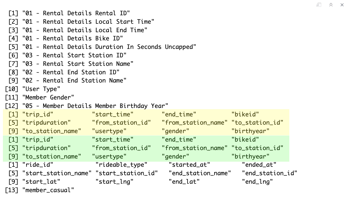
Great! Looks like 2019 Q3 and Q4 have the most common column names. Let’s match the column names now.
#Standardize column names in 2019 Q2 and 2020 Q1 dataframes
DT_2019_Q2 <- plyr::rename(Divvy_Trips_2019_Q2, c('01 - Rental Details Rental ID' = 'trip_id',
         '01 - Rental Details Duration In Seconds Uncapped' = 'tripduration',
         '01 - Rental Details Local Start Time' = 'start_time',
         '01 - Rental Details Local End Time' = 'end_time',
         '03 - Rental Start Station ID' = 'from_station_id',
         '03 - Rental Start Station Name' = 'from_station_name',
         '02 - Rental End Station ID' = 'to_station_id',
         '02 - Rental End Station Name' = 'to_station_name',
         'User Type' = 'usertype'))

DT_2020_Q1 <- plyr::rename(Divvy_Trips_2020_Q1, c('ride_id' = 'trip_id',
         'start_station_id' = 'from_station_id',
         'started_at' = 'start_time',
         'ended_at' = 'end_time',
         'start_station_name' = 'from_station_name',
         'end_station_id' = 'to_station_id',
         'end_station_name' = 'to_station_name',
         'member_casual' = 'usertype'))

#Create dataframes for 2019 Q3 and 2019 Q4
DT_2019_Q3 <- Divvy_Trips_2019_Q3
DT_2019_Q4 <- Divvy_Trips_2019_Q4
Add the missing ‘tripduration’ column to DT_2020_Q1.
#Load package
library(lubridate)

#Add trip duration column
DT_2020_Q1 <- DT_2020_Q1 %>%
  mutate(tripduration = as.numeric(difftime(end_time, start_time, units = 'secs')))
Then select relevant columns for analysis.
DT_2019_Q2_df <- DT_2019_Q2 %>%
  select('trip_id', 'start_time', 'end_time', 'tripduration', 'from_station_id', 'from_station_name', 'to_station_id', 'to_station_name', 'usertype')

DT_2019_Q3_df <- DT_2019_Q3 %>%
  select('trip_id', 'start_time', 'end_time', 'tripduration', 'from_station_id', 'from_station_name', 'to_station_id', 'to_station_name', 'usertype')

DT_2019_Q4_df <- DT_2019_Q4 %>%
  select('trip_id', 'start_time', 'end_time', 'tripduration', 'from_station_id', 'from_station_name', 'to_station_id', 'to_station_name', 'usertype')

DT_2020_Q1_df <- DT_2020_Q1 %>%
  select('trip_id', 'start_time', 'end_time', 'tripduration', 'from_station_id', 'from_station_name', 'to_station_id', 'to_station_name', 'usertype')
Add a column to designate quarter-year in each dataframe.
DT_2019_Q2_df <- DT_2019_Q2_df %>%
  mutate(quarter_year = 'Q2_2019')

DT_2019_Q3_df <- DT_2019_Q3_df %>%
  mutate(quarter_year = 'Q3_2019')

DT_2019_Q4_df <- DT_2019_Q4_df %>%
  mutate(quarter_year = 'Q4_2019')

DT_2020_Q1_df <- DT_2020_Q1_df %>%
  mutate(quarter_year = 'Q1_2020')
Now combine the dataframes.
DT_all <- rbind(DT_2019_Q2_df, DT_2019_Q3_df, DT_2019_Q4_df, DT_2020_Q1_df)
Separate DateTime column to date and time columns.
DT_all <- tidyr::separate(DT_all, start_time, c('start_date', 'start_time'), sep = ' ')
DT_all <- tidyr::separate(DT_all, end_time, c('end_date', 'end_time'), sep = ' ')
Check the data structure with glimpse.
glimpse(DT_all)
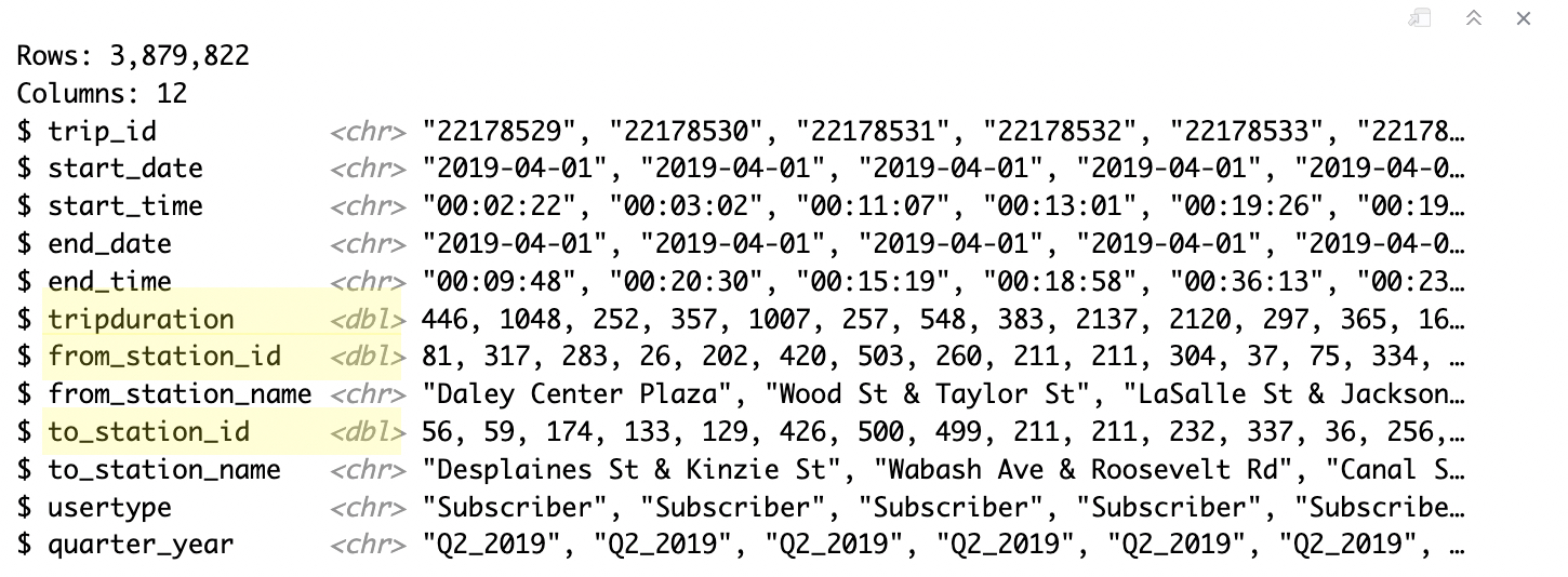
Looks like ‘tripduration’, ‘from_station_id’, and ‘to-station-id’ are the wrong data classes. Let’s fix that.
as.character(DT_all$from_station_id)
as.character(DT_all$to_station_id)
as.numeric(DT_all$tripduration)
Time to add more date columns to improve analysis granularity.
DT_all$date <- as.Date(DT_all$start_date) #The default format is yyyy-mm-dd
DT_all$month <- format(as.Date(DT_all$date), "%m")
DT_all$day <- format(as.Date(DT_all$date), "%d")
DT_all$year <- format(as.Date(DT_all$date), "%Y")
DT_all$day_of_week <- format(as.Date(DT_all$date), "%A")

DT_all <- DT_all %>%
  mutate(hour = hour(hms(start_time)))
Let’s get rid of the rest of the ‘bad’ data. We’ll drop the start and end date columns.
drop <- c('start_date', 'end_date')
DT_all_v2 <- DT_all[!(names(DT_all) %in% drop)]
Then remove duplicates and NAs.
DT_all_v2 <- DT_all_v2[!duplicated(DT_all_v2$trip_id), ]
DT_all_v2 <- na.omit(DT_all_v2)
Standardize usertype column to match stakeholder definitions.
unique(DT_all_v2$usertype)
DT_all_v2$usertype[DT_all_v2$usertype=='Subscriber'] <- 'member'
DT_all_v2$usertype[DT_all_v2$usertype=='Customer'] <- 'casual'
Check if stakeholder’s HQ is present in the data.
DT_all_v2[grep('HQ', DT_all_v2$from_station_name), ]
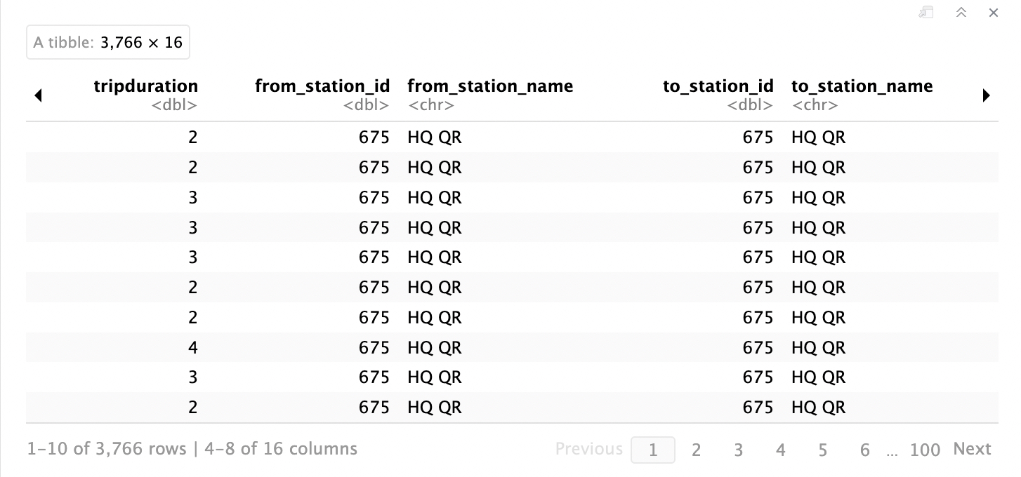
Yup, the HQ is included in the data. What about negative values in the trip duration column?
min(DT_all_v2$tripduration)

Yikes, there are trips with negative durations. Let’s remove HQ and the negative values from the data.
DT_all_v3 <- DT_all_v2[!(DT_all_v2$from_station_name == 'HQ QR' | DT_all_v2$tripduration<0),]
That’s much better! Time for analysis!
Descriptive Analysis
First make sure that days of week are ordered properly.
DT_all_v3$day_of_week <- ordered(DT_all_v3$day_of_week, levels=c('Sunday', 'Monday', 'Tuesday', 'Wednesday', 'Thursday', 'Friday', 'Saturday'))
Use the aggregate function to compare trip duration for user types.
aggregate(DT_all_v3$tripduration~DT_all_v3$usertype, FUN = summary)
Then use aggregate functions to get descriptive statistics of various levels of date granularity (date, month, year, hour, etc.).
aggregate(DT_all_v3$tripduration~DT_all_v3$usertype + DT_all_v3$date-type, FUN = summary)
Now for the fun part! Time to analyze the trip count by user type and date/time granularity.
#Count trips by user type
user_count <- DT_all_v3 %>%
  group_by(usertype) %>%
  dplyr::summarise(total_count=n(),.groups='drop')

#Count trips by user type and weekday
user_count_wkd <- DT_all_v3 %>%
  group_by(usertype, day_of_week) %>%
  dplyr::summarise(total_count=n(),.groups='drop')
user_count_wkd_w <- spread(user_count_wkd, day_of_week, total_count)

#Count trips weekly average
trip_cnt_wkd_avg_mem <- user_count_wkd %>%
  filter(user_count_wkd$usertype == 'member') %>%
  dplyr::summarise(avg_wkd = mean(total_count),.groups='drop')

trip_cnt_wkd_avg_c <- user_count_wkd %>%
  filter(user_count_wkd$usertype == 'casual') %>%
  dplyr::summarise(avg_wkd = mean(total_count),.groups='drop')

#Count trips by user type and hour
user_count_hr <- DT_all_v3 %>%
  group_by(usertype, hour) %>%
  dplyr::summarise(total_count=n(),.groups='drop')
user_count_hr_w <- spread(user_count_hr, usertype, total_count)

#Count trips by user type and quarter
user_count_q <- DT_all_v3 %>%
  group_by(usertype, quarter_year) %>%
  dplyr::summarise(total_count=n(),.groups='drop')
user_count_q_w <- spread(user_count_q, quarter_year, total_count)

#Count trips by user type and month
user_count_month <- DT_all_v3 %>%
  group_by(usertype, month) %>%
  dplyr::summarise(total_count=n(),.groups='drop')
user_count_month_w <- spread(user_count_month, month, total_count)
And now for trip duration averages.
#Average duration by user type (min)
user_td_avg <- DT_all_v3 %>%
  group_by(usertype) %>%
  dplyr::summarise(avg_tripduration_min = (mean(tripduration)/60))

#Average tripduration by user type and weekday (min)
user_wkd_avg <- DT_all_v3 %>%
  group_by(usertype, day_of_week) %>%
  dplyr::summarise(avg_tripduration_min = (mean(tripduration)/60),.groups='drop')
user_wkd_avg_w <- spread(user_wkd_avg, day_of_week, avg_tripduration_min)
All set with this phase of the analysis!
Data is ready to be exported and uploaded into Tableau to create visualizations!
write.csv(DT_all_v3, file = 'DT_all_v3.csv')
Analysis Summary & Visualizations
For an interactive walkthrough of the data analysis and dashboards visit the data story on Tableau!
How do member trips compare to casual trips yearly? (Q2 2019 - Q1 2020)
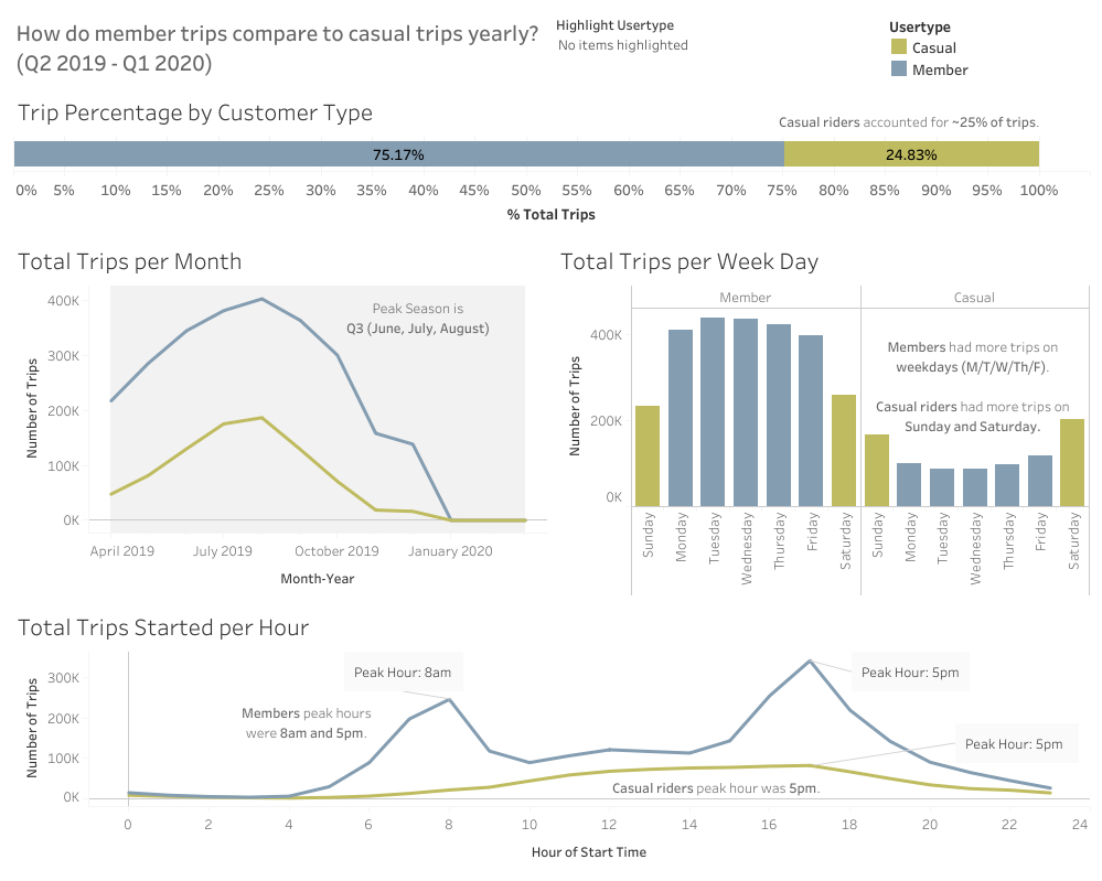
Percentages
- Casual riders made 25% of the trips.
- Members made 75% of the trips.
Peak Times
- There is a peak season for trips in the third quarter, in June, July, and August.
- Casual riders used bikes more often on weekends (Sat/Sun).
- Members used bikes more often on weekdays (Mon/Tue/Wed/Thu/Fri).
Most Popular Starting Hour
- Most casual riders start trips at 5pm.
- Most members start trips at 8am and 5pm.
What is the most popular trip start time during Q3 2019 (peak months) for members and casual riders?
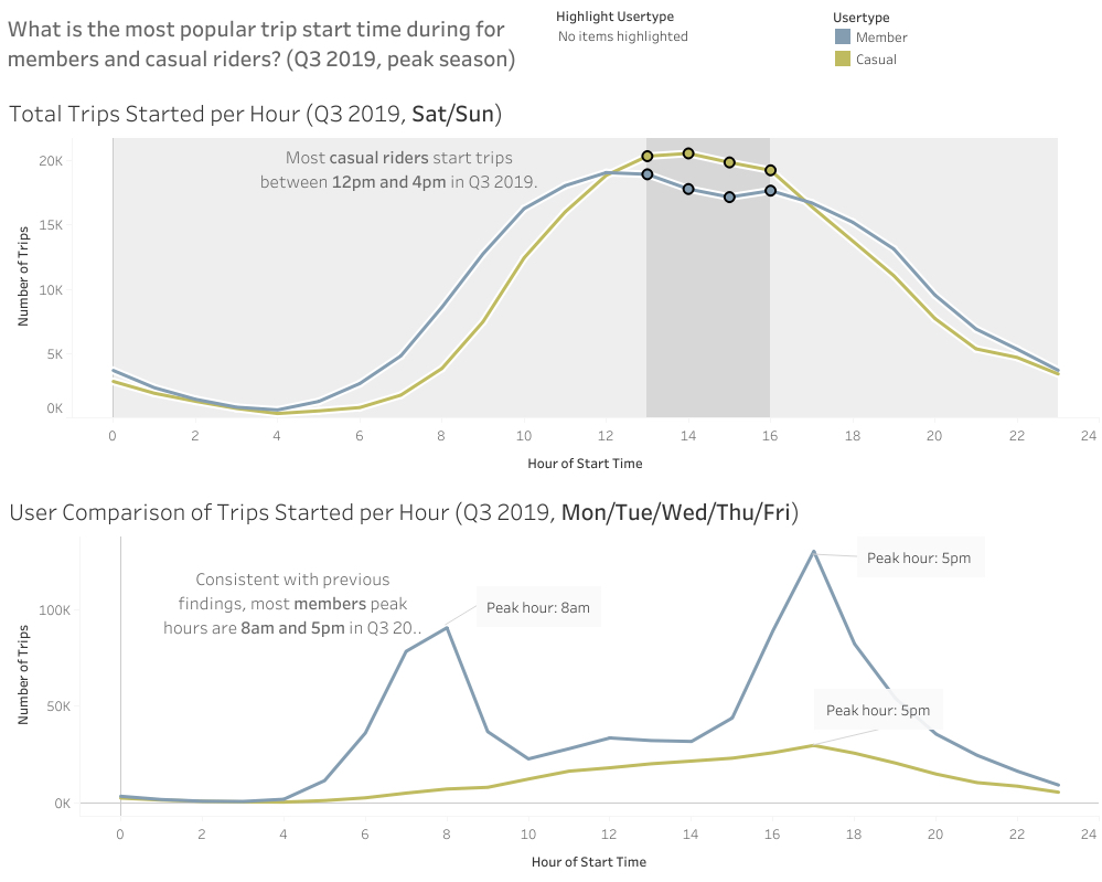
- Most casual riders start trips between 12pm and 4pm on weekends (Sat/Sun).
- Most member trips start at 8am or at 5pm on week days (Mon/Tue/Wed/Thu/Fri).
How do member and casual trip durations compare yearly?
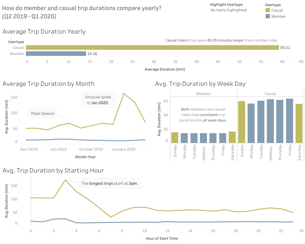
Average Trip Duration
- Casual riders have longer trips than members (59.2 min > 14.2 min).
- There was an unusual average trip duration spike of 161.6 min in January 2020. Further investigation of this time period is recommended.
- Average trip duration was consistent weekly for both members and casual riders.
- The longest trips for both members and casual riders started at 3am.
Recommendations for Marketing Campaign
A quick recap on the Stakeholder Goal:
Cyclistic aims to increase its number of annual memberships by targeting casual members through a marketing campaign.
Recommendations:
- Target weekday casual riders in peak season (Q3)
- Send promotions at 8am & 5pm to encourage commuter-member signups
- Create a discount reward system to encourage larger quantities of short trips
- Increase number of bikes available at 5pm to meet the growing demand
- Target weekend casual riders in peak season (Q3)
- Send promotions on Thursday & Friday at 5pm to encourage weekend-member signups
- Use weekend adventure imagery for marketing campaign
- Create sightseeing suggestions perk for members only